What is Naive Bayes ??
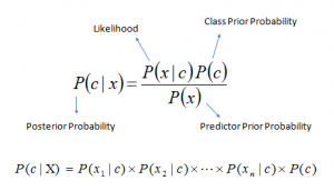
According to scikit - learn.org Naive Bayes methods are a set of supervised learning algorithms that are based on Bayes Theorem with the ‘naive’ assumption that there is a conditional independence between every pair of features given the value of class variable.

Where:
-
P(c x) is the posterior probability of class (c, target) given predictor (x, attributes). -
P(c) is the prior probability of class. -
P(x c) is the likelihood which is the probability of predictor given class. -
P(x) is the prior probability of predictor.
There are three types of Naive Bayes Algorithms:
1. Gaussian Naive Bayes This algorithm follows the Gaussian Normal distribution and supports continuous data with the assumption that the continous values associated with each class are distributed according to a normal (or Gaussian) distribution.
2. Multinominal Naive Bayes This algorithm is suitable for classification with dicrete features (word counts for text classicification for example) it normally requires integer feature counts, however fractional counts such as tf-idf may work as well.
3. Bernoulli Naive Bayes This algorithm is similar to multinominal naive bayes however, in a Bernoulli Naive Bayes, the predictors are boolean variables (yes or no) rather than integers.
Main advantages of Naive Bayes are that :
- fast and easy to understand
- not prone to overfitting
- performs well with small amounts of data
- when the assumption holds to be true, it performs better compared to other models such as logisitic regression
Some disadvantages of Navie Bayes are that:
- does not work very well when the number of featrues is very high
- the assumption that input features are independent of each other may not always hold to be true
- important imformation may be lost while resampling the continous variables
This post today will focus on the Gaussian Naive Bayes algorithm. We will build one from scratch to gain a better understanding of the model.
Step 1 - Instantiate the Class:
import numpy as np

class GaussianNBClassifier:
    def __init__(self):
        pass
Step 2 - Seperate By Class
We need to find the base rate - or the probability of data by the class they belong to, so we need to seperate our training data by class.
def separate_classes(self, X, y):
    separated_classes = {}
    for i in range(len(X)):
        feature_values = X[i]
        class_name = y[i]
        if class_name not in separated_classes:
            separated_classes[class_name] = []
        separated_classes[class_name].append(feature_values)
    return separated_classes
Step 3 - Summarize Features
We will create a summary for each feature in the dataset because the probability is assumed to be Gaussion and is calculated based on the mean and standard deviation.
def summarize(self, X):
    for feature in zip(*X):
        yield {
            'stdev' : np.std(feature),
            'mean' : np.mean(feature)
        }
Step 4 - Gaussian Distribution Function
We use the Gaussian Distribution Function (GDF) to find the probability for features following a normal distribution
def gauss_distribution_function(self, x, mean, stdev):
    exponent = np.exp(-((x-mean)**2 / (2*stdev**2)))
    return exponent / (np.sqrt(2*np.pi)*stdev)
Step 5 - Train the Model
By training our model, we are telling it to learn from the dataset. With Gaussian Bayes Classifier, this involves calculating the mean and standard deviation for each feature os each class. This allows us to then calculate the probability we will use for predictions.
def fit(self, X, y):
    separated_classes = self.separate_classes(X, y)
    self.class_summary = {}
    for class_name, feature_values in separated_classes.items():
        self.class_summary[class_name] = {
            'prior_proba': len(feature_values)/len(X),
            'summary': [i for i in self.summarize(feature_values)],
        }
    return self.class_summary
Step 6 - Make Predictions
In order for us to predict a class, we have to calculate the posterior probability for each one. The class which has the highest posterior probability will then be the predicted class.
The posterior probability is calculated by dividing the joint probability by the mariginal probability
The mariginal probability (denominator) is the total joint probability of all classes
The joint probability is the numerator of the fraction used to calculate the posterior probability:
We can then select the class with the maximum value for the joint probability
joint_proba = {}
for class_name, features in self.class_summary.items():
    total_features = len(features['summary'])
    likelihood = 1
    for idx in range(total_features):
        feature = row[idx]
        mean = features['summary'][idx]['mean']
        stdev = features['summary'][idx]['stdev']
        normal_proba = self.gauss_distribution_function(feature, mean, stdev)
        likelihood *= normal_proba
    prior_proba = features['prior_proba']
    joint_proba[class_name] = prior_proba * likelihood
Step 7 - Putting It All Together
We can now predict the class for each row in our test data set:
def predict(self, X):
    MAPs = []
    for row in X:
        joint_proba = {}
        for class_name, features in self.class_summary.items():
            total_features = len(features['summary'])
            likelihood = 1
            for idx in range(total_features):
                feature = row[idx]
                mean = features['summary'][idx]['mean']
                stdev = features['summary'][idx]['stdev']
                normal_proba = self.gauss_distribution_function(feature, \
                mean, stdev)
                likelihood *= normal_proba
            prior_proba = features['prior_proba']
            joint_proba[class_name] = prior_proba * likelihood
        MAP = max(joint_proba, key=joint_proba.get)
        MAPs.append(MAP)
    return MAPs
Step 8 - Calculate the Accuracy
To test our model’s performance, we will divide the number of correct predictions by the total number of predicitions, which will then give us the models accuracy
def accuracy(self, y_test, y_pred):
    true_true = 0
    for y_t, y_p in zip(y_test, y_pred):
        if y_t == y_p:
            true_true += 1
    return true_true / len(y_test)
Comparing
Now lets compare our from scratch model’s performance with the performance of the Gaussian model from scikit - learn using the UCI Wine data set
GaussianNBClassifier
from GaussianNBClassifier import GaussianNBClassifier

model = GaussianNBClassifier()
model.fit(X_train, y_train)
y_pred = model.predict(X_test)
print ("GaussianNBClassifier accuracy: {0:.3f}".format(model.accuracy(y_test, y_pred)))
Output:
GaussianNBClassifier accuracy: 0.972
Scikit-learn GaussianNB
from sklearn.naive_bayes import GaussianNB
from sklearn.metrics import accuracy_score

model = GaussianNB()
model.fit(X_train, y_train)
y_pred = model.predict(X_test)
print ("Scikit-learn GaussianNB accuracy: {0:.3f}".format(accuracy_score(y_test, y_pred)))
Output:
Scikit-learn GaussianNB accuracy: 0.972
The accuracy of our from scratch model matches the accuracy from the scikit-learn model, meaning we have implemented a successful Gaussian Naive Bayes model from scratch !!
References
- https://scikit-learn.org/stable/modules/naive_bayes.html
- https://www.mathsisfun.com/data/bayes-theorem.html
- https://www.analyticsvidhya.com/blog/2017/09/naive-bayes-explained/
- https://machinelearningmastery.com/naive-bayes-classifier-scratch-python/

